Chaos Theory: Tent Map (Part 1)

In previous posts regarding chaos theory we have investigated the logistic map. In this post we’re going to be looking at a similar system known as the tent map; it is also commonly referred to as the triangle map.

The tent map is a recurrence relation, written as:

for   and .

As shown below, the graph of has maximum value at . The tent map is piecewise linear, because of this characteristic this makes the tent map easier to analyse than the logistic map. However, although the form of the tent map is simple and the equations are linear, for certain parameter values the map can yield complex and chaotic behaviour [1].

Tent map

The logistic and tent map are topologically conjugate for and respectively. In other words, the behaviour of the tent map for is the same as that of the logistic map when . The proof of this is will be looked at in future posts. First lets look to see if the tent map is sensitive to initial conditions. Here we’ll use similar initial conditions to that found in previous posts for the logistic map; and and

Tent map: Sensitivity to Initial Conditions

Similarly to the logistic map, we can see that the tent map is also sensitive to initial conditions. In addition to being sensitive to initial conditions, the tent map is also dependent on its parameter value , ranging from predictable to chaotic behaviour. We will explore the tent map further in the next post.

Sources:

[1] LYNCH, S. (2007). Dynamical Systems with Applications Using Mathematica (eBook). Birkhäuser Basel, 1st edition.

Chaos Theory: Dependence on parameter r (continued)

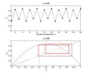
Previously we looked at how the logistic map is affected by changing the parameter r for small values. Now we’re going to look at what happens when we change it the parameter r for large values, say . Instead of converging to a fixed point, the orbit oscillates. For the logistic map, these orbits exist between and and the oscillations repeat every two iterations as shown below:

Period-2 orbits

This is also known as a period-2 orbit. Again, for larger values of r, say , the orbit now repeats its oscillations every four iterations.

Period-4 orbits

In other words, the previous orbit has doubled its period to a period-4 orbit. The splitting of the orbit is known as a bifurcation, i.e. at the orbit bifurcates into two solutions, and for the orbit bifurcates into four solutions. As we increase r even further, more bifurcations occur resulting in orbits of period . The table below shows values of r for which these bifurcations occur [1].

We can graph this data to get the bifurcation diagram for the logistic map, showing the possible long-term behaviour for all values of r between 0 and 4. Note, you can click on the image to see a larger version of the image.

Bifurcation for r between 0 and 4

To clarify and understand the points of bifurcations; we can also graph the bifurcation at a smaller interval for r.

Zoomed in of the above bifurcation. Values of r between r=2.8 and r=4.0

Clearly from both the table and graphs we can observe that the bifurcations occur faster and faster until . Here the map becomes chaotic and has infinite number of periodic orbits. Therefore, an infinite set of points or solutions. In other words, the map doesn’t converge to a fixed point or periodic orbit, instead it becomes aperiodic. This is an example into the periodic-doubling route to chaos. We can plot histograms with reference to the bifurcation diagrams. The histograms display the amount of time a typical orbit spends in some part of the attractor, for different values of r we have different attractors. Here we’ll use 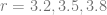and , with initial condition 0.4 and 10000 x values. From the bifurcation diagrams we expect that the distribution of data eventually spreads across the whole range of x values (0 to 1) as we increase the parameter r.

Logistic map histograms: Distribution of data

For , the data lies on two values which supports the fact that for the orbit is period-2, and so the orbit oscillates between two values. Similarly for , the orbit is period-4 and the data lies on four values. As we approach we begin to see the data converging to a U-shaped distribution, with the number of values intensifying at zero and one.

Sources:

[1] STROGATZ, S.H. (1994). Nonlinear dynamics and chaos. New York, USA. Westview Press, Perseus.

(I suggest you check this book out, it’s amazing and helped me a lot through my university years)!

P.S. All images generated on MATLAB, if you want my M-files then feel free to contact me!

Chaos Theory: Dependence on parameter r.

In the previous post on chaos theory we looked at the logistic map, a simple 1-D discrete map which illustrates chaotic behaviour.  This map was defined by the following equation:

.

We’re going to be looking at the maps dependence upon the parameter value r. The logistic map shows a wide range of different behaviours depending upon our choice of r. Here we’ll be using initial condition . As we can see in the figure below, for  the orbit tends to 0, independent of the initial condition. However, when the orbit will quickly converge towards a fixed point. For clarity we will connect the discrete points by line segments, note, only the blue points are significant, using initial condition throughout. The population is decreasing and will eventually approach 0 as the number of iterations tends to infinity for the map tends to 0. For we can show mathematically that the population approaches a fixed point .

Logistic map orbit for various r values.

Using (1) then the fixed points are when . Expanding gives , we then divide through by to get  and finally rearrange to get fixed point at . For example, at the fixed point is at . These results can be supported by plotting the corresponding cobweb plots (also seen below).

Logistic map: corresponding cobweb plots for various r values.

In the next post about chaos theory, we’re going to be investigating what happens when we look at higher values of r, alongside introducing ways of representing all the data onto one plot. We get some remarkable images when we do this!

As previously stated, all plots are made via MATLAB, if you wish to acquire the MATLAB codes, feel free to contact me!

Chaos Theory: Sensitivity to Initial Conditions

As stated in the previous posts, sensitivity to initial conditions is popularly known as the butterfly effect. It is one of the properties of chaos theory mostly affiliated by scientists when determining if a given system is chaotic. It means that each point in a system is arbitrarily closely approximated by other points with distinguishably different orbits in the future. In other words, a small change to the initial conditions may lead to significantly different behaviour. However, just because systems are sensitive to initial conditions it doesn’t imply that they are chaotic. To illustrate we will look at the mapping given below:

Starting at two initial conditions and with minute differences the orbits diverge quickly from one another. Starting with a small difference of approximately 0.01 after 10 iterations. However, after 20 iterations, the difference is in its billions. The graph above shows the map between 14 and 19 iterations with the orbits represented by different colours, red and blue. Clearly, the system is dependent on initial conditions, however, the system isn’t chaotic. The distinction of chaotic systems is that, given two states that are minute in difference, the orbits distance from one another continuously varies; i.e. sometimes becoming arbitrarily close or far from one another with respect to the attractor. For the quadratic system, this doesn’t occur, and so, it isn’t chaotic. To illustrate this we will look at the logistic map for different initial conditions.

Like before we represent the two orbits of the logistic map with different colours (graph above) . As shown, the orbits remain the same for the first few iterations. However, eventually the orbits diverge from each other and become non-identical, and so exhibit behaviour of sensitivity to initial conditions. To support this we plot the corresponding (absolute) distance between the orbits. In contrast to the quadratic mapping before, the difference between the two orbits vary. Clearly, the difference is arbitrarily small sometimes and then arbitrarily large with respect to the attractor, and so demonstrates behaviour of a chaotic system. Note the rate at which nearby orbits diverge from each other with time is characterised by a statistic called the Lyapunov exponent. This helps determine chaotic behaviour, and is a statistic we will be looking at later in the blog.

Chaos Theory: Logistic Map Introduction

This chapter looks at dynamical systems where by time is discrete. These systems are also known as iterated maps or difference equations. In particular, we will be focusing on 1-D dynamical systems, when plotted the orbit is just a sequence of points in the real numbers (). The two systems we will be looking at (as previously stated) are the logistic map and the tent map, these maps illustrate how chaotic behaviour arises from simple systems.

The logistic map was first proposed to describe the dynamics of insect populations by biologist Robert May in 1976. Often speculated as the archetypal example of how chaotic behaviour arises from simple dynamical equations, it is a recurrence relation, written as

where represents the ratio of the existing populations to a possible maximum population at year n such that . For example,  represents the initial ratio at year 0. The parameter r is a positive number, representing the rate of reproduction and starvation such that .

The graph of (1) is a parabola with maximum value of r/4 at  as shown above. Increasing the value of r=0 to r=4 make the map undergo a series of period-doubling bifurcations, something we will be exploring later on. The logistic map has fixed points at x=0 and x=1, regardless of r. However, the stability of the fixed points depend upon r. Again, something we will be exploring in the future.

P.S. All graphical output produced on MATLAB.